HW8
Sarah Stover
2025-03-19
Partner: Sydney Miller
Simulating and Fitting Data Distributions
Loading the data and libraries: The data set we are using measures Honeybee hygenic behavior scores (a continuous dataset)
library(dplyr)

z <- read.csv("UBO_DataSheet.csv",header=TRUE,sep=",")
z <- z %>%
  select(field_ID, assay_score) %>%
  filter(!is.na(assay_score))%>%
#changing any 0s to small non-0 numbers in a different column
  mutate(myVar = ifelse(assay_score == 0, 0.0001, assay_score))

colnames(z) <- c("ID", "Var", "myVar")

library(ggplot2) # for graphics
library(MASS) # for maximum likelihood estimation
##
## Attaching package: 'MASS'## The following object is masked from 'package:dplyr':
##
## select# quick and dirty, a truncated normal distribution to work on the solution set
#z <- rnorm(n=3000,mean=0.2)
#z <- data.frame(1:3000,z)
#names(z) <- list("ID","myVar")
#z <- z[z$myVar>0,]
#str(z)
#summary(z$myVar)Plot histogram of the data
p1 <- ggplot(data=z, aes(x=myVar, y=..density..)) +
  geom_histogram(color="grey60",fill="cornsilk",size=0.2)
print(p1)
## Warning: The dot-dot notation (`..density..`) was
## deprecated in ggplot2 3.4.0.
## ℹ Please use `after_stat(density)` instead.
## This warning is displayed once every 8 hours.
## Call `lifecycle::last_lifecycle_warnings()` to
## see where this warning was generated.## `stat_bin()` using `bins = 30`. Pick better
## value with `binwidth`.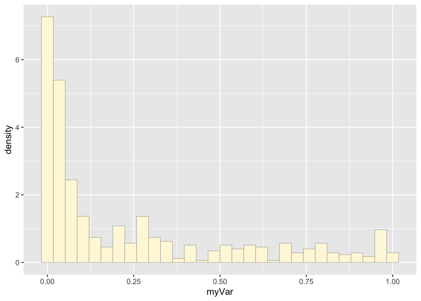
#adds an empirical density curve
p1 <-  p1 +  geom_density(linetype="dotted",size=0.75)
print(p1)
## `stat_bin()` using `bins = 30`. Pick better
## value with `binwidth`.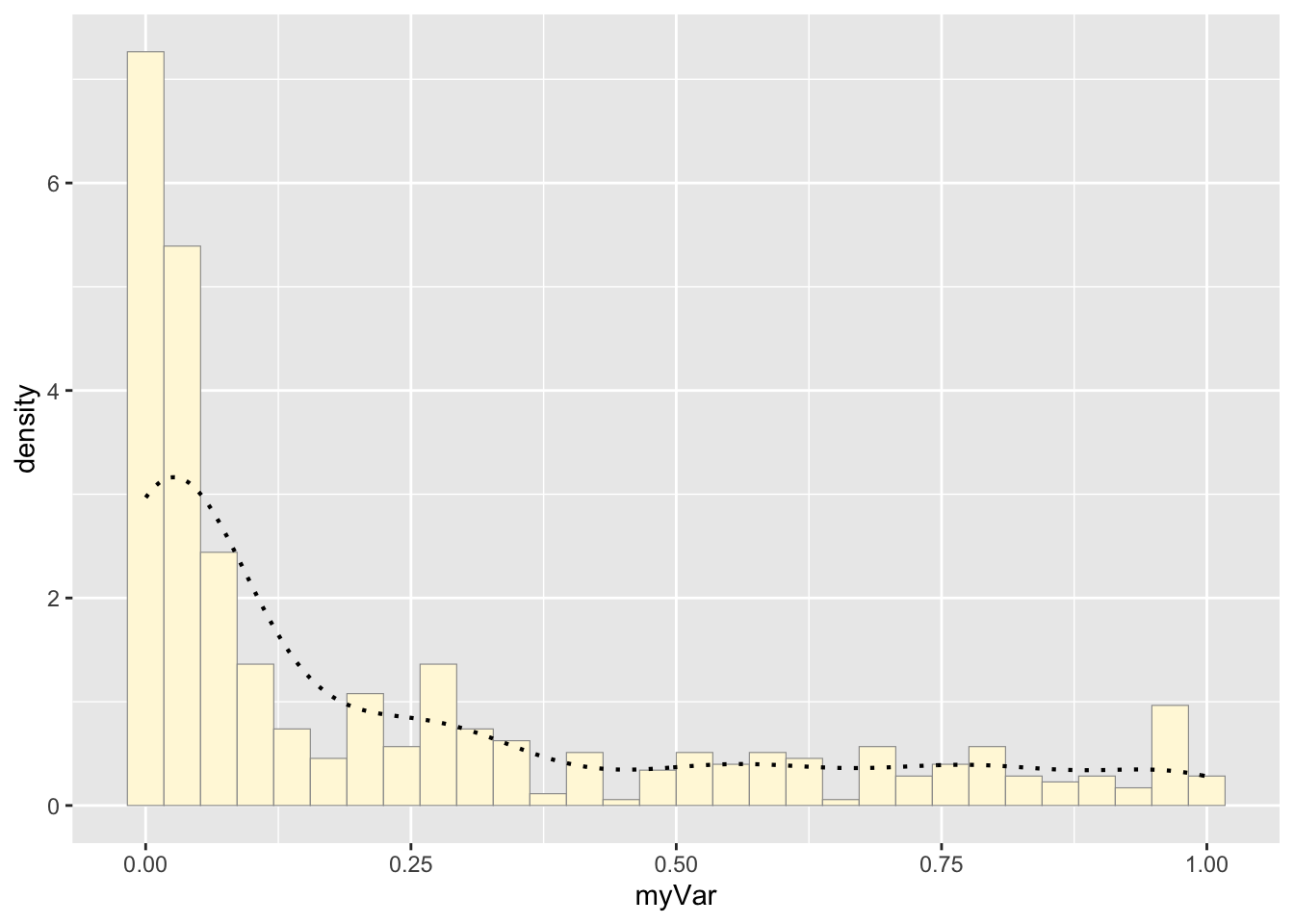
#get maximum likelihood parameters for normal distribution
normPars <- fitdistr(z$myVar,"normal")
print(normPars)
## mean sd
## 0.233664971 0.297085812
## (0.013142303) (0.009293011)str(normPars)## List of 5
## $ estimate: Named num [1:2] 0.234 0.297
## ..- attr(*, "names")= chr [1:2] "mean" "sd"
## $ sd : Named num [1:2] 0.01314 0.00929
## ..- attr(*, "names")= chr [1:2] "mean" "sd"
## $ vcov : num [1:2, 1:2] 1.73e-04 0.00 0.00 8.64e-05
## ..- attr(*, "dimnames")=List of 2
## .. ..$ : chr [1:2] "mean" "sd"
## .. ..$ : chr [1:2] "mean" "sd"
## $ n : int 511
## $ loglik : num -105
## - attr(*, "class")= chr "fitdistr"normPars$estimate["mean"] # note structure of getting a named attribute## mean
## 0.233665Plot normal probability density, can use stat function to generate probability density
meanML <- normPars$estimate["mean"]
sdML <- normPars$estimate["sd"]

xval <- seq(0,max(z$myVar),len=length(z$myVar))

 stat <- stat_function(aes(x = xval, y = ..y..), fun = dnorm, colour="red", n = length(z$myVar), args = list(mean = meanML, sd = sdML))
 p1 + stat
## `stat_bin()` using `bins = 30`. Pick better
## value with `binwidth`.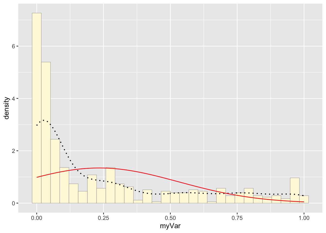
Plot exponential probability density
expoPars <- fitdistr(z$myVar,"exponential")
rateML <- expoPars$estimate["rate"]

stat2 <- stat_function(aes(x = xval, y = ..y..), fun = dexp, colour="blue", n = length(z$myVar), args = list(rate=rateML))
 p1 + stat + stat2
## `stat_bin()` using `bins = 30`. Pick better
## value with `binwidth`.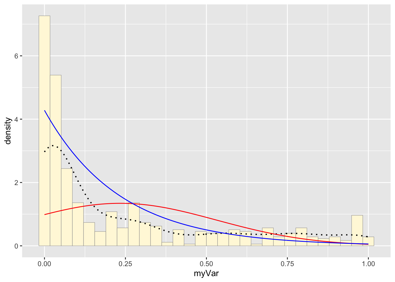
Plot uniform density probability
 stat3 <- stat_function(aes(x = xval, y = ..y..), fun = dunif, colour="darkgreen", n = length(z$myVar), args = list(min=min(z$myVar), max=max(z$myVar)))
 p1 + stat + stat2 + stat3
## `stat_bin()` using `bins = 30`. Pick better
## value with `binwidth`.
Plot gamma probability density
gammaPars <- fitdistr(z$myVar,"gamma")## Warning in densfun(x, parm[1], parm[2], ...): NaNs produced
## Warning in densfun(x, parm[1], parm[2], ...): NaNs produced
## Warning in densfun(x, parm[1], parm[2], ...): NaNs produced
## Warning in densfun(x, parm[1], parm[2], ...): NaNs produced
## Warning in densfun(x, parm[1], parm[2], ...): NaNs produced
## Warning in densfun(x, parm[1], parm[2], ...): NaNs produced
## Warning in densfun(x, parm[1], parm[2], ...): NaNs produced
## Warning in densfun(x, parm[1], parm[2], ...): NaNs produced
## Warning in densfun(x, parm[1], parm[2], ...): NaNs produced
## Warning in densfun(x, parm[1], parm[2], ...): NaNs produced
## Warning in densfun(x, parm[1], parm[2], ...): NaNs produced
## Warning in densfun(x, parm[1], parm[2], ...): NaNs produced
## Warning in densfun(x, parm[1], parm[2], ...): NaNs produced
## Warning in densfun(x, parm[1], parm[2], ...): NaNs produced
## Warning in densfun(x, parm[1], parm[2], ...): NaNs producedshapeML <- gammaPars$estimate["shape"]
rateML <- gammaPars$estimate["rate"]
stat4 <- stat_function(aes(x = xval, y = ..y..), fun = dgamma, colour="brown", n = length(z$myVar), args = list(shape=shapeML, rate=rateML))
p1 + stat + stat2 + stat3 + stat4## `stat_bin()` using `bins = 30`. Pick better
## value with `binwidth`.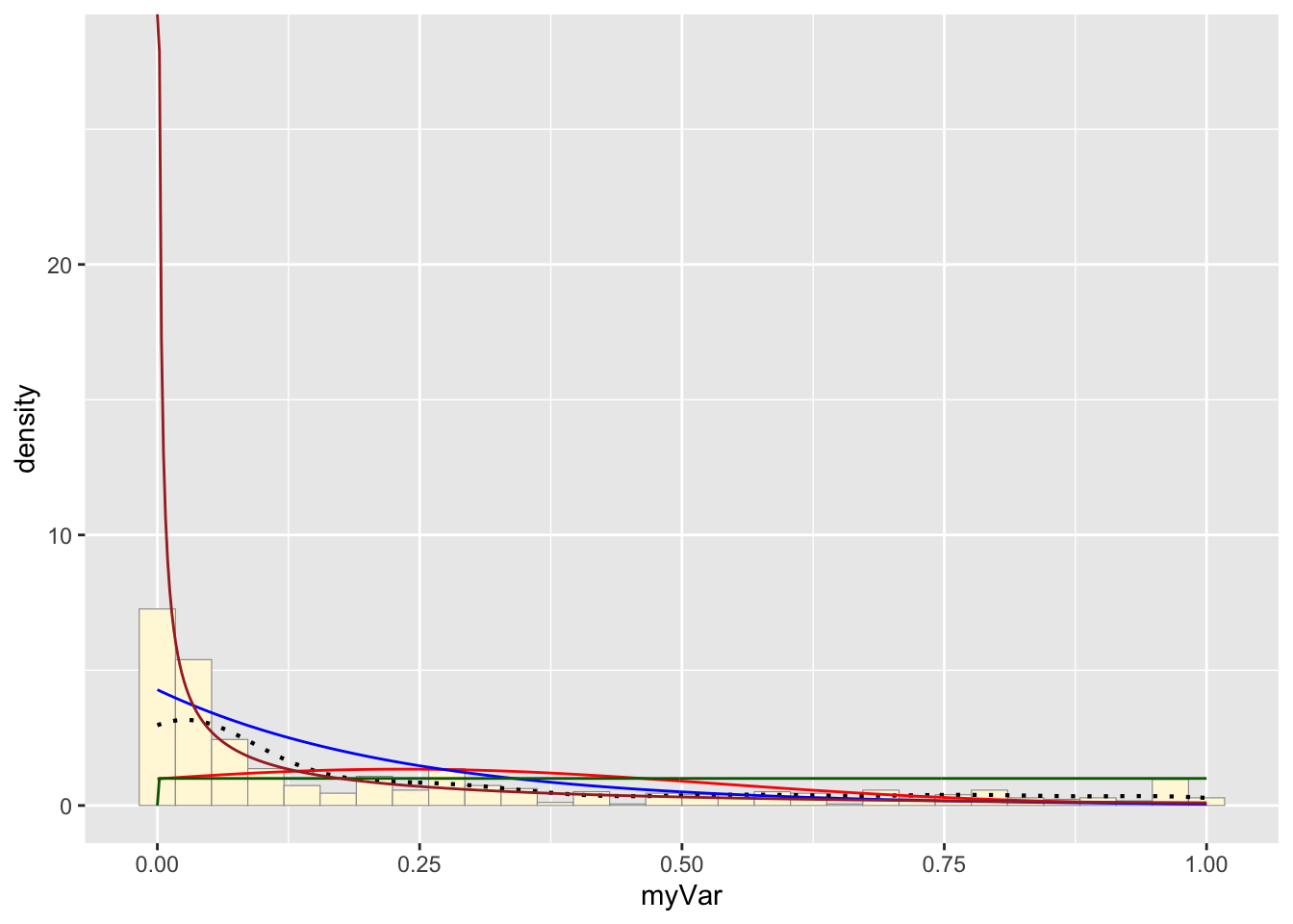
Plot beta probability density
 pSpecial <- ggplot(data=z, aes(x=myVar/(max(myVar + 0.1)), y=..density..)) +
  geom_histogram(color="grey60",fill="cornsilk",size=0.2) +
  xlim(c(0,1)) +
  geom_density(size=0.75,linetype="dotted")

betaPars <- fitdistr(x=z$myVar/max(z$myVar + 0.1),start=list(shape1=1,shape2=2),"beta")
## Warning in densfun(x, parm[1], parm[2], ...): NaNs produced
## Warning in densfun(x, parm[1], parm[2], ...): NaNs produced
## Warning in densfun(x, parm[1], parm[2], ...): NaNs produced
## Warning in densfun(x, parm[1], parm[2], ...): NaNs produced
## Warning in densfun(x, parm[1], parm[2], ...): NaNs produced
## Warning in densfun(x, parm[1], parm[2], ...): NaNs produced
## Warning in densfun(x, parm[1], parm[2], ...): NaNs produced
## Warning in densfun(x, parm[1], parm[2], ...): NaNs produced
## Warning in densfun(x, parm[1], parm[2], ...): NaNs producedshape1ML <- betaPars$estimate["shape1"]
shape2ML <- betaPars$estimate["shape2"]
statSpecial <- stat_function(aes(x = xval, y = ..y..), fun = dbeta, colour="orchid", n = length(z$myVar), args = list(shape1=shape1ML,shape2=shape2ML))
pSpecial + statSpecial## `stat_bin()` using `bins = 30`. Pick better
## value with `binwidth`.## Warning: Removed 2 rows containing missing values or
## values outside the scale range (`geom_bar()`).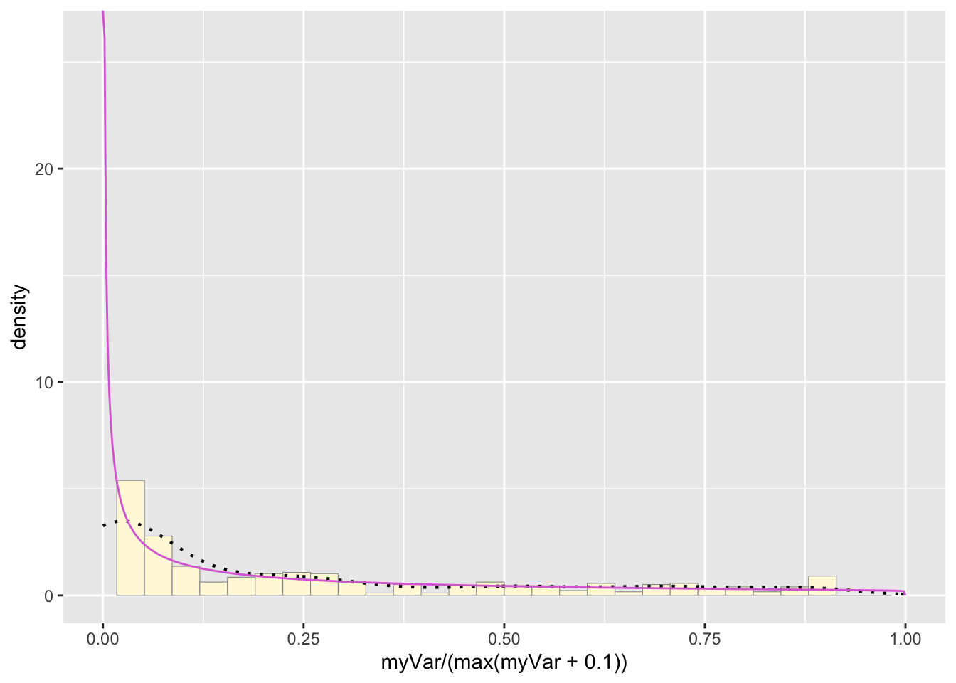 Which Probability Curve is the best fit?
Based on all of the fit lines, I think that the gamma and exponential probability distributions fit the best. The beta distribution is likely too close to infinity at 0 to really fit our data set but both the gamma and exponential probability distributions are quite similar. This makes sense as the exponential distribution is part of the family of gamma probability distribution, just a special case of it. If we want to distinguish between these two curves to see what fits the hive hygenic behavior stats, More sampling is needed to get a higher resolution of the probability distribution.