HW6
Sarah Stover
2025-02-19
Data Set Information and Summary:
For this homework, we are working with survey data of beekeepers in Vermont who are members VBA (Vermont Beekeepers Association). In this dataset they rated or commented their satisfation with certain areas of the organization. We want to understand the demographics of VBA and how the organization’s resources are allotted. Who is needs more support and how can we be more inclusive to minorities or new beekeepers. Instead of generating our own data, we just built a nested forloop to go through the dataset and look at different categories.
#uploading and reading the data frame, getting
df <- read.csv("Annual Survey Results - 2025 Winter meeting.csv")
#exploring the df
head(df)
## Annual_meetings Mentorship_program Access_resources
## 1 Satisfied No prior experience Neutral
## 2 Satisfied No prior experience Very satisfied
## 3 Very satisfied Satisfied
## 4 Very satisfied No prior experience No prior experience
## 5 No prior experience No prior experience Very satisfied
## 6 No prior experience No prior experience No prior experience
## Educational_workshops Industry_policy_insights Networking_opportunities
## 1 Neutral Satisfied Satisfied
## 2 Very satisfied Satisfied Satisfied
## 3 Satisfied Satisfied Very satisfied
## 4 No prior experience No prior experience Very satisfied
## 5 Very satisfied Very satisfied No prior experience
## 6 No prior experience No prior experience No prior experience
## News_updates Marketing_social
## 1 Satisfied Satisfied
## 2 Satisfied Satisfied
## 3 Satisfied Satisfied
## 4 Very satisfied Very satisfied
## 5 Very satisfied No prior experience
## 6 No prior experience No prior experience
## Option_to_explain Speaker.Name.s..
## 1 NA
## 2 NA
## 3 NA
## 4 Cant sign onto website as a member to renew membership NA
## 5 NA
## 6 NA
## Topic.s.. Speaker.Category
## 1
## 2
## 3
## 4 Types of hives pros & cons Hive management techniques
## 5
## 6
## Workshop.Topic.s..
## 1
## 2
## 3 Making nucs, overwinter splits
## 4 Types of hives pros & cons
## 5 Beginner beekeeping, treating for mites
## 6 First time beekeeping
## Workshop.Category Age Gender Race
## 1 55-64 Male White
## 2 35-54 Male White
## 3 Preparing for winter, Hive management techniques 65+ Male White
## 4 Hive management techniques 55-64 Male White
## 5 Pests and pathogens 65+ Female White
## 6 Hive management techniques
## Location Scale Beekeeping_experience
## 1 Southern Vermont Hobbyist Beekeeper (<25 colonies) 10+
## 2 Northwest Vermont Hobbyist Beekeeper (<25 colonies) 4-6
## 3 Western Vermont Hobbyist Beekeeper (<25 colonies) 4-6
## 4 Other Sideliner Beekeeper (25-300 colonies) 4-6
## 5 Central Vermont Hobbyist Beekeeper (<25 colonies) 0-3
## 6Looking at Gendered differences in satisfaction between all organization categories:
library(dplyr)##
## Attaching package: 'dplyr'## The following objects are masked from 'package:stats':
##
## filter, lag## The following objects are masked from 'package:base':
##
## intersect, setdiff, setequal, unionlibrary(tidyr)
proportion_results <- list()
# Loop through each gender (Male and Female)
for (gender in c("Male", "Female")) {
# Subset the data for this gender group
gender_data <- df[df$Gender == gender, ]
# Initialize a list to store proportions for this gender
gender_proportions <- list()
# Loop through each relevant column (Annual_meeting and Mentorship_programs)
for (column in c("Annual_meetings", "Mentorship_program", "Access_resources", "Educational_workshops", "Industry_policy_insights", "Networking_opportunities", "News_updates", "Marketing_social")) {
# Calculate the proportion of each category for this column
prop_very_satisfied <- mean(gender_data[[column]] == "Very satisfied") * 100
prop_satisfied <- mean(gender_data[[column]] == "Satisfied") * 100
prop_unsatisfied <- mean(gender_data[[column]] == "Unsatisfied") * 100
prop_very_unsatisfied <- mean(gender_data[[column]] == "Very unsatisfied") * 100
prop_neutral <- mean(gender_data[[column]] == "Neutral") * 100
prop_noexperience <- mean(gender_data[[column]] == "No prior experience") * 100
# Store the results in the list for this column
gender_proportions[[column]] <- c("Very satisfied" = prop_very_satisfied,
"Satisfied" = prop_satisfied,
"Unsatisfied" = prop_unsatisfied,
"Very unsatisfied" = prop_very_unsatisfied,
"Neutral" = prop_neutral,
"No prior expreience" = prop_noexperience)
}
# Store the results for this gender
proportion_results[[gender]] <- gender_proportions
}
# Print the results
print(proportion_results)## $Male
## $Male$Annual_meetings
## Very satisfied Satisfied Unsatisfied Very unsatisfied
## 36.842105 31.578947 0.000000 0.000000
## Neutral No prior expreience
## 5.263158 26.315789
##
## $Male$Mentorship_program
## Very satisfied Satisfied Unsatisfied Very unsatisfied
## 15.789474 5.263158 5.263158 0.000000
## Neutral No prior expreience
## 0.000000 63.157895
##
## $Male$Access_resources
## Very satisfied Satisfied Unsatisfied Very unsatisfied
## 31.578947 36.842105 0.000000 0.000000
## Neutral No prior expreience
## 5.263158 21.052632
##
## $Male$Educational_workshops
## Very satisfied Satisfied Unsatisfied Very unsatisfied
## 52.631579 21.052632 0.000000 0.000000
## Neutral No prior expreience
## 5.263158 15.789474
##
## $Male$Industry_policy_insights
## Very satisfied Satisfied Unsatisfied Very unsatisfied
## 42.10526 26.31579 0.00000 0.00000
## Neutral No prior expreience
## 10.52632 15.78947
##
## $Male$Networking_opportunities
## Very satisfied Satisfied Unsatisfied Very unsatisfied
## 47.368421 26.315789 0.000000 0.000000
## Neutral No prior expreience
## 5.263158 15.789474
##
## $Male$News_updates
## Very satisfied Satisfied Unsatisfied Very unsatisfied
## 31.57895 47.36842 0.00000 0.00000
## Neutral No prior expreience
## 0.00000 15.78947
##
## $Male$Marketing_social
## Very satisfied Satisfied Unsatisfied Very unsatisfied
## 31.57895 36.84211 0.00000 0.00000
## Neutral No prior expreience
## 15.78947 10.52632
##
##
## $Female
## $Female$Annual_meetings
## Very satisfied Satisfied Unsatisfied Very unsatisfied
## 9.090909 27.272727 0.000000 0.000000
## Neutral No prior expreience
## 9.090909 45.454545
##
## $Female$Mentorship_program
## Very satisfied Satisfied Unsatisfied Very unsatisfied
## 27.272727 0.000000 9.090909 9.090909
## Neutral No prior expreience
## 9.090909 27.272727
##
## $Female$Access_resources
## Very satisfied Satisfied Unsatisfied Very unsatisfied
## 27.272727 36.363636 0.000000 9.090909
## Neutral No prior expreience
## 9.090909 9.090909
##
## $Female$Educational_workshops
## Very satisfied Satisfied Unsatisfied Very unsatisfied
## 54.545455 27.272727 0.000000 9.090909
## Neutral No prior expreience
## 0.000000 0.000000
##
## $Female$Industry_policy_insights
## Very satisfied Satisfied Unsatisfied Very unsatisfied
## 36.363636 0.000000 0.000000 9.090909
## Neutral No prior expreience
## 18.181818 18.181818
##
## $Female$Networking_opportunities
## Very satisfied Satisfied Unsatisfied Very unsatisfied
## 27.272727 18.181818 9.090909 9.090909
## Neutral No prior expreience
## 9.090909 9.090909
##
## $Female$News_updates
## Very satisfied Satisfied Unsatisfied Very unsatisfied
## 63.636364 0.000000 9.090909 9.090909
## Neutral No prior expreience
## 0.000000 0.000000
##
## $Female$Marketing_social
## Very satisfied Satisfied Unsatisfied Very unsatisfied
## 27.272727 18.181818 0.000000 9.090909
## Neutral No prior expreience
## 18.181818 18.181818# Create a new column that indicates whether a person is unsatisfied or not
df$Mentorship_programClean <- ifelse(df$Mentorship_program %in% c("Unsatisfied", "Very Unsatisfied", "Neutral"), "Unsatisfied", "Satisfied")
# Create a contingency table for gender vs unsatisfaction status
contingency_table <- table(df$Gender, df$Mentorship_programClean)
# Perform the Chi-squared test
chi_squared_test <- chisq.test(contingency_table)## Warning in chisq.test(contingency_table): Chi-squared approximation may be
## incorrect# Print the results of the test
print(chi_squared_test)##
## Pearson's Chi-squared test
##
## data: contingency_table
## X-squared = 6.3283, df = 2, p-value = 0.04225print(contingency_table)##
## Satisfied Unsatisfied
## 7 5
## Female 9 2
## Male 18 1Because we are working with categorical values, we used a chi square analysis instead of ANOVA. Based on the p value (0.042) we can say there is a gendered difference between satisfaction levels.
Who is not coming to networking events by gender?:
#library(ggplot2

#removes NAs, mutates original dataset, creates a new column called networking_attendance. Then looks at df$Networking_opportunities to see if the answer is "no prior experience". if this is TRUE then its "did not attend" in the new column. Anything else is "Attended".
library(ggplot2)

df <- df %>%
  #filtering out NAs in Netwoking and Gender columns
  filter(!is.na(Networking_opportunities) & !is.na(Gender) & Gender != "") %>%
  mutate(Networking_attendance = ifelse(Networking_opportunities == "No prior experience", "Did Not Attend", "Attended"))

ggplot(df, aes(x = Gender, fill = Networking_attendance)) +
  geom_bar(position = "dodge") + #side by side bars
  labs(title = "Networking Opportunity Attendence by Gender", x = "Gender", y = "count") + scale_fill_manual(values = c("Attended"= "pink", "Did Not Attend" = "orange"))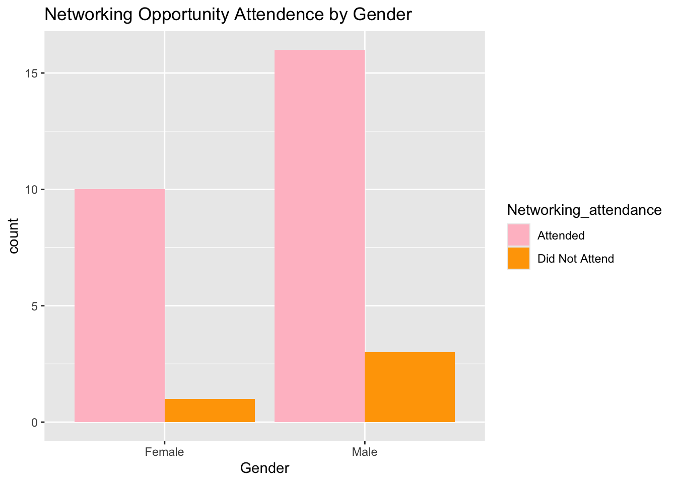
NetworkOpp_by_Gender_table <- table(df$Gender, df$Networking_attendance)
print(NetworkOpp_by_Gender_table)
##
## Attended Did Not Attend
## Female 10 1
## Male 16 3There doesn’t seem to be a bias in who is attending networking events by gender. The next thing to explore is by years of experience. Are those with less experience attending more or less than those already established?
Participation in Networking Events by Beekeeping Experience:
# Create a new column that indicates whether a person is unsatisfied or not
df$Networking_opportunitiesClean <- ifelse(df$Networking_opportunities %in% c("Unsatisfied", "Very Unsatisfied", "Neutral"),  "Unsatisfied", "Satisfied")

# Create a contingency table for gender vs unsatisfaction status
contingency_table2 <- table(df$Beekeeping_experience, df$Networking_opportunitiesClean)

print(contingency_table2)
##
## Satisfied Unsatisfied
## 0-3 7 1
## 10+ 6 1
## 4-6 10 1
## 7-10 4 0# Perform the Chi-squared test
chi_squared_test2 <- chisq.test(contingency_table2)## Warning in chisq.test(contingency_table2): Chi-squared approximation may be
## incorrect# Print the results of the test
print(chi_squared_test2)##
## Pearson's Chi-squared test
##
## data: contingency_table2
## X-squared = 0.65296, df = 3, p-value = 0.8842# Get the standardized residuals
standardized_residuals2 <- chi_squared_test2$stdres
#Priint residuals
print(standardized_residuals2)##
## Satisfied Unsatisfied
## 0-3 -0.2752409 0.2752409
## 10+ -0.4316658 0.4316658
## 4-6 0.1262892 -0.1262892
## 7-10 0.7161149 -0.7161149Based on the Chi square value, there no significant satisfaction based on years of experience.